SIAMCAT input files formats
Konrad Zych, Jakob Wirbel, and Georg Zeller
EMBL Heidelberggeorg.zeller@embl.de
Date last modified: 2018-09-24
SIAMCAT_read-in.RmdIntroduction
This vignette illustrates how to read and input your own data to the
SIAMCAT package. We will cover reading in text files from
the disk, formatting them and using them to create an object of
siamcat-class.
The siamcat-class is the centerpiece of the package. All
of the input data and result are stored inside of it. The structure of
the object is described below in the siamcat-class object section.
Loading your data into R
SIAMCAT input
Generally, there are three types of input for
SIAMCAT:
Features
The features should be a matrix, a
data.frame, or an otu_table, organized as
follows:
features (in rows) x samples (in columns).
| Sample_1 | Sample_2 | Sample_3 | Sample_4 | Sample_5 | |
|---|---|---|---|---|---|
| Feature_1 | 0.59 | 0.71 | 0.78 | 0.61 | 0.66 |
| Feature_2 | 0.00 | 0.02 | 0.00 | 0.00 | 0.00 |
| Feature_3 | 0.02 | 0.00 | 0.00 | 0.00 | 0.20 |
| Feature_4 | 0.34 | 0.00 | 0.13 | 0.07 | 0.00 |
| Feature_5 | 0.06 | 0.16 | 0.00 | 0.00 | 0.00 |
Please note that
SIAMCATis supposed to work with relative abundances. Other types of data (e.g. counts) will also work, but not all functions of the package will result in meaningful outputs.
An example of a typical feature file is attached to the
SIAMCAT package, containing data from a publication
investigating the microbiome in colorectal cancer (CRC) patients and
controls (the study can be found here: Zeller et al). The
metagenomics data were processed with the MOCAT pipeline, returning taxonomic
profiles on the species levels (specI):
library(SIAMCAT)
fn.in.feat  <- system.file(
    "extdata",
    "feat_crc_zeller_msb_mocat_specI.tsv",
    package = "SIAMCAT"
)
One way to load such data into R could be the use of
read.table
(Beware of the defaults in R! They are not always useful…)
feat <- read.table(fn.in.feat, sep='\t',
    header=TRUE, quote='',
    stringsAsFactors = FALSE, check.names = FALSE)
# look at some features
feat[110:114, 1:2]
## CCIS27304052ST-3-0 CCIS15794887ST-4-0
## Bacteroides caccae [h:1096] 1.557937e-03 1.761949e-03
## Bacteroides eggerthii [h:1097] 2.734527e-05 4.146882e-05
## Bacteroides stercoris [h:1098] 1.173786e-03 2.475838e-03
## Bacteroides clarus [h:1099] 4.830533e-04 4.589747e-06
## Methanohalophilus mahii [h:11] 0.000000e+00 0.000000e+00Metadata
The metadata should be either a matrix or a
data.frame.
samples (in rows) x metadata (in columns):
| Age | Gender | BMI | |
|---|---|---|---|
| Sample_1 | 52 | 1 | 20 |
| Sample_2 | 37 | 1 | 18 |
| Sample_3 | 66 | 2 | 24 |
| Sample_4 | 54 | 2 | 26 |
| Sample_5 | 65 | 2 | 30 |
The rownames of the metadata should match the
colnames of the feature matrix.
Again, an example of such a file is attached to the
SIAMCAT package, taken from the same study:
fn.in.meta  <- system.file(
    "extdata",
    "num_metadata_crc_zeller_msb_mocat_specI.tsv",
    package = "SIAMCAT"
)
Also here, the read.table can be used to load the data
into R.
meta <- read.table(fn.in.meta, sep='\t',
    header=TRUE, quote='',
    stringsAsFactors = FALSE, check.names = FALSE)
head(meta)
## age gender bmi diagnosis localization crc_stage fobt
## CCIS27304052ST-3-0 52 1 20 0 NA 0 0
## CCIS15794887ST-4-0 37 1 18 0 NA 0 0
## CCIS74726977ST-3-0 66 2 24 1 NA 0 0
## CCIS16561622ST-4-0 54 2 26 0 NA 0 0
## CCIS79210440ST-3-0 65 2 30 0 NA 0 1
## CCIS82507866ST-3-0 57 2 24 0 NA 0 0
## wif_test
## CCIS27304052ST-3-0 0
## CCIS15794887ST-4-0 0
## CCIS74726977ST-3-0 NA
## CCIS16561622ST-4-0 0
## CCIS79210440ST-3-0 0
## CCIS82507866ST-3-0 0Label
Finally, the label can come in different three different flavours:
-
Named vector: A named vector containing information about cases and controls. The names of the vector should match the
rownamesof the metadata and thecolnamesof the feature data. The label can contain either the information about cases and controls either- as integers (e.g.
0and1), - as characters (e.g.
CTRandIBD), or - as factors.
- as integers (e.g.
Metadata column: You can provide the name of a column in the metadata for the creation of the label. See below for an example.
-
Label file:
SIAMCAThas a function calledread.label, which will create a label object from a label file. The file should be organized as follows:- The first line is supposed to read:
#BINARY:1=[label for cases];-1=[label for controls] - The second row should contain the sample identifiers as tab-separated list (consistent with feature and metadata).
- The third row is then supposed to contain the actual class labels
(tab-separated):
1for each case and-1for each control.
An example file is attached to the package again, if you want to have a look at it.
- The first line is supposed to read:
For our example dataset, we can create the label object out of the
metadata column called diagnosis:
label <- create.label(meta=meta, label="diagnosis",
    case = 1, control=0)
When we later plot the results, it might be nicer to have names for
the different groups stored in the label object (instead of
1 and 0). We can also supply them to the
create.label function:
label <- create.label(meta=meta, label="diagnosis",
    case = 1, control=0,
    p.lab = 'cancer', n.lab = 'healthy')
## Label used as case:
## 1
## Label used as control:
## 0## + finished create.label.from.metadata in 0.001 s
label$info## healthy cancer
## -1 1Note:
If you have no label information for your dataset, you can still create aSIAMCATobject from your features alone. TheSIAMCATobject without label information will contain aTESTlabel that can be used for making holdout predictions. Other functions, e.g. model training, will not work on such an object.
LEfSe format files
LEfSe is a tool for identification of associations between micriobial features and up to two metadata. LEfSe uses LDA (linear discriminant analysis).
LEfSe input file is a .tsv file. The first few rows
contain the metadata. The following row contains sample names and the
rest of the rows are occupied by features. The first column holds the
row names:
| label | healthy | healthy | healthy | cancer | cancer |
|---|---|---|---|---|---|
| age | 52 | 37 | 66 | 54 | 65 |
| gender | 1 | 1 | 2 | 2 | 2 |
| Sample_info | Sample_1 | Sample_2 | Sample_3 | Sample_4 | Sample_5 |
| Feature_1 | 0.59 | 0.71 | 0.78 | 0.61 | 0.66 |
| Feature_2 | 0.00 | 0.02 | 0.00 | 0.00 | 0.00 |
| Feature_3 | 0.02 | 0.00 | 0.00 | 0.00 | 0.00 |
| Feature_4 | 0.34 | 0.00 | 0.43 | 0.00 | 0.00 |
| Feature_5 | 0.56 | 0.56 | 0.00 | 0.00 | 0.00 |
An example of such a file is attached to the SIAMCAT
package:
fn.in.lefse<- system.file(
    "extdata",
    "LEfSe_crc_zeller_msb_mocat_specI.tsv",
    package = "SIAMCAT"
)
SIAMCAT has a dedicated function to read LEfSe format
files. The read.lefse function will read in the input file
and extract metadata and features:
meta.and.features <- read.lefse(fn.in.lefse,
    rows.meta = 1:6, row.samples = 7)
meta <- meta.and.features$meta
feat <- meta.and.features$feat
We can then create a label object from one of the columns of the meta
object and create a siamcat object:
label <- create.label(meta=meta, label="label", case = "cancer")## Label used as case:
## cancer
## Label used as control:
## healthy## + finished create.label.from.metadata in 0.049 smetagenomeSeq format files
metagenomeSeq is an R package to determine differentially abundant features between multiple samples.
There are two ways to input data into metagenomeSeq:
- two files, one for metadata and one for features - those can be used
in
SIAMCATjust like described in SIAMCAT input withread.table:
fn.in.feat  <- system.file(
    "extdata",
    "CHK_NAME.otus.count.csv",
    package = "metagenomeSeq"
)
feat <- read.table(fn.in.feat, sep='\t',
    header=TRUE, quote='', row.names = 1,
    stringsAsFactors = FALSE, check.names = FALSE
)-
BIOMformat file, that can be used inSIAMCATas described in the following section
BIOM format files
The BIOM format files can be added to SIAMCAT via
phyloseq. First the file should be imported using the
phyloseq function import_biom. Then a
phyloseq object can be imported as a siamcat
object as descibed in the next
section.
Creating a siamcat object of a phyloseq object
The siamcat object extends on the phyloseq
object. Therefore, creating a siamcat object from a
phyloseq object is really straightforward. This can be done
with the siamcat constructor function. First, however, we
need to create a label object:
data("GlobalPatterns") ## phyloseq example data
label <- create.label(meta=sample_data(GlobalPatterns),
    label = "SampleType",
    case = c("Freshwater", "Freshwater (creek)", "Ocean"))
## Label used as case:
## Freshwater,Freshwater (creek),Ocean
## Label used as control:
## rest## + finished create.label.from.metadata in 0.003 s
# run the constructor function
siamcat <- siamcat(phyloseq=GlobalPatterns, label=label)
## + starting validate.data## +++ checking overlap between labels and features## + Keeping labels of 26 sample(s).## +++ checking sample number per class## Data set has a limited number of training examples:
## rest 18
## Case 8
## Note that a dataset this small/skewed is not necessarily suitable for analysis in this pipeline.## +++ checking overlap between samples and metadata## + finished validate.data in 0.264 sCreating a siamcat-class object
The siamcat-class is the centerpiece of the package. All
of the is stored inside of the object: 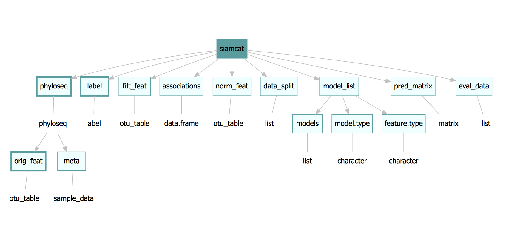
In the figure above, rectangles depict slots of the object and the
class of the object stored in the slot is given in the ovals. There are
two obligatory slots -phyloseq (containing the metadata
as sample_data and the original features as
otu_table) and label - marked with thick
borders.
The siamcat object is constructed using the
siamcat() function. There are two ways to initialize
it:
-
Features: You can provide a feature
matrix,data.frame, orotu_tableto the function (together with label and metadata information):siamcat <- siamcat(feat=feat, label=label, meta=meta) -
phyloseq: The alternative is to create a
siamcatobject directly out of aphyloseqobject:siamcat <- siamcat(phyloseq=phyloseq, label=label)
Please note that you have to provide either
feat or phyloseq and that you
cannot provide both.
In order to explain the siamcat object better we will
show how each of the slots is filled.
phyloseq, label and orig_feat slots
The phyloseq and label slots are obligatory.
- The phyloseq slot is an object of class
phyloseq, which is described in the help file of thephyloseqclass. Help can be accessed by typing into R console:help('phyloseq-class').- The
otu_tableslot inphyloseq-seehelp('otu_table-class')- stores the original feature table. ForSIAMCAT, this slot can be accessed byorig_feat.
- The
- The label slot contains a list. This list has a specific set of
entries -see
help('label-class')- that are automatically generated by theread.labelorcreate.labelfunctions.
The phyloseq, label and orig_feat are filled when the
siamcat object is first created with the constructor
function. 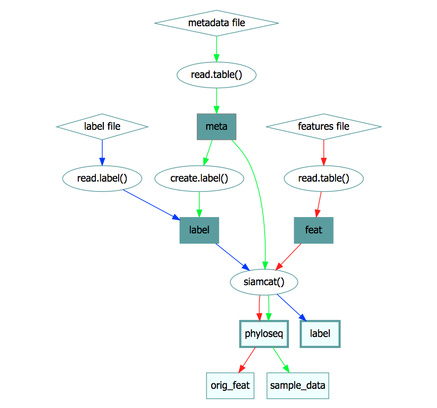
Accessing and assigning slots
Each slot in siamcat can be accessed by typing
slot_name(siamcat)e.g. for the eval_data slot you can types
eval_data(siamcat)There is one notable exception: the phyloseq slot has to be accessed
with physeq(siamcat) due to technical reasons.
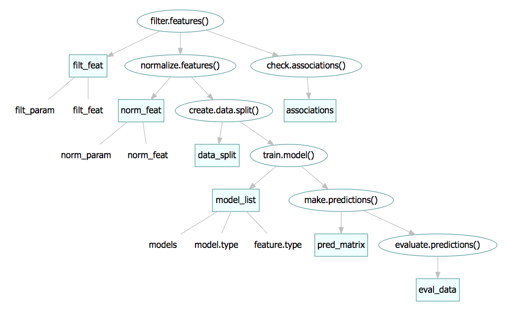
Slots will be filled during the SIAMCAT workflow by the
package’s functions. However, if for any reason a slot needs to be
assigned outside of the workflow, the following formula can be used:
slot_name(siamcat) <- object_to_assigne.g. to assign a new_label object to the
label slot:
label(siamcat) <- new_labelPlease note that this may lead to unforeseen consequences…
Slots inside the slots
There are two slots that have slots inside of them. First, the
model_list slot has a models slot that
contains the actual list of mlr
models -can be accessed via models(siamcat)- and
model.type which is a character with the name of the method
used to train the model: model_type(siamcat).
The phyloseq slot has a complex structure. However, unless the
phyloseq object is created outside of the SIAMCAT workflow,
only two slots of phyloseq slot will be occupied: the
otu_table slot containing the features table and the
sam_data slot containing metadata information. Both can be
accessed by typing either features(siamcat) or
meta(siamcat).
Additional slots inside the phyloseq slots do not have dedicated
accessors, but can easily be reached once the phyloseq object is
exported from the siamcat object:
## Taxonomy Table:     [6 taxa by 7 taxonomic ranks]:
##        Kingdom   Phylum          Class          Order          Family
## 549322 "Archaea" "Crenarchaeota" "Thermoprotei" NA             NA
## 522457 "Archaea" "Crenarchaeota" "Thermoprotei" NA             NA
## 951    "Archaea" "Crenarchaeota" "Thermoprotei" "Sulfolobales" "Sulfolobaceae"
## 244423 "Archaea" "Crenarchaeota" "Sd-NA"        NA             NA
## 586076 "Archaea" "Crenarchaeota" "Sd-NA"        NA             NA
## 246140 "Archaea" "Crenarchaeota" "Sd-NA"        NA             NA
##        Genus        Species
## 549322 NA           NA
## 522457 NA           NA
## 951    "Sulfolobus" "Sulfolobusacidocaldarius"
## 244423 NA           NA
## 586076 NA           NA
## 246140 NA           NA
If you want to find out more about the phyloseq data structure, head over to the phyloseq BioConductor page. # Session Info
## R version 4.2.2 (2022-10-31)
## Platform: x86_64-apple-darwin17.0 (64-bit)
## Running under: macOS Big Sur ... 10.16
##
## Matrix products: default
## BLAS:   /Library/Frameworks/R.framework/Versions/4.2/Resources/lib/libRblas.0.dylib
## LAPACK: /Library/Frameworks/R.framework/Versions/4.2/Resources/lib/libRlapack.dylib
##
## locale:
## [1] en_US.UTF-8/en_US.UTF-8/en_US.UTF-8/C/en_US.UTF-8/en_US.UTF-8
##
## attached base packages:
## [1] stats     graphics  grDevices utils     datasets  methods   base
##
## other attached packages:
## [1] SIAMCAT_2.3.3    phyloseq_1.42.0  mlr3_0.14.1      BiocStyle_2.26.0
##
## loaded via a namespace (and not attached):
##   [1] paradox_0.11.0         minqa_1.2.5            colorspace_2.1-0
##   [4] ellipsis_0.3.2         rprojroot_2.0.3        XVector_0.38.0
##   [7] fs_1.6.1               rstudioapi_0.14        listenv_0.9.0
##  [10] mlr3tuning_0.18.0      fansi_1.0.4            codetools_0.2-19
##  [13] splines_4.2.2          mlr3learners_0.5.6     PRROC_1.3.1
##  [16] cachem_1.0.7           knitr_1.42             ade4_1.7-22
##  [19] jsonlite_1.8.4         nloptr_2.0.3           pROC_1.18.0
##  [22] gridBase_0.4-7         cluster_2.1.4          BiocManager_1.30.20
##  [25] compiler_4.2.2         backports_1.4.1        Matrix_1.5-3
##  [28] fastmap_1.1.1          cli_3.6.0              prettyunits_1.1.1
##  [31] htmltools_0.5.4        tools_4.2.2            lmerTest_3.1-3
##  [34] igraph_1.4.1           gtable_0.3.1           glue_1.6.2
##  [37] GenomeInfoDbData_1.2.9 reshape2_1.4.4         LiblineaR_2.10-22
##  [40] dplyr_1.1.0            Rcpp_1.0.10            Biobase_2.58.0
##  [43] jquerylib_0.1.4        pkgdown_2.0.7          vctrs_0.5.2
##  [46] Biostrings_2.66.0      rhdf5filters_1.10.0    multtest_2.54.0
##  [49] ape_5.7-1              nlme_3.1-162           iterators_1.0.14
##  [52] xfun_0.37              stringr_1.5.0          globals_0.16.2
##  [55] lme4_1.1-32            lifecycle_1.0.3        beanplot_1.3.1
##  [58] future_1.32.0          zlibbioc_1.44.0        MASS_7.3-58.3
##  [61] scales_1.2.1           lgr_0.4.4              hms_1.1.2
##  [64] ragg_1.2.5             parallel_4.2.2         biomformat_1.26.0
##  [67] rhdf5_2.42.0           RColorBrewer_1.1-3     yaml_2.3.7
##  [70] memoise_2.0.1          gridExtra_2.3          ggplot2_3.4.1
##  [73] sass_0.4.5             stringi_1.7.12         S4Vectors_0.36.2
##  [76] desc_1.4.2             corrplot_0.92          foreach_1.5.2
##  [79] checkmate_2.1.0        permute_0.9-7          palmerpenguins_0.1.1
##  [82] BiocGenerics_0.44.0    boot_1.3-28.1          shape_1.4.6
##  [85] GenomeInfoDb_1.34.9    matrixStats_0.63.0     rlang_1.1.0
##  [88] pkgconfig_2.0.3        systemfonts_1.0.4      bitops_1.0-7
##  [91] evaluate_0.20          lattice_0.20-45        purrr_1.0.1
##  [94] Rhdf5lib_1.20.0        tidyselect_1.2.0       parallelly_1.34.0
##  [97] plyr_1.8.8             magrittr_2.0.3         bookdown_0.33
## [100] R6_2.5.1               IRanges_2.32.0         generics_0.1.3
## [103] DBI_1.1.3              pillar_1.8.1           mgcv_1.8-42
## [106] survival_3.5-5         RCurl_1.98-1.10        tibble_3.2.0
## [109] crayon_1.5.2           uuid_1.1-0             utf8_1.2.3
## [112] rmarkdown_2.20         progress_1.2.2         grid_4.2.2
## [115] data.table_1.14.8      vegan_2.6-4            infotheo_1.2.0.1
## [118] mlr3misc_0.11.0        bbotk_0.7.2            digest_0.6.31
## [121] numDeriv_2016.8-1.1    textshaping_0.3.6      stats4_4.2.2
## [124] munsell_0.5.0          glmnet_4.1-6           bslib_0.4.2