Meta-analysis using SIAMCAT
Jakob Wirbel, and Georg Zeller
EMBL Heidelberggeorg.zeller@embl.de
Date last modified: 2020-11-05
SIAMCAT_meta.RmdAbout This Vignette
In this vignette, we want to demonstrate how SIAMCAT can
facilitate metagenomic meta-analyses, focussing both on association
testing and ML workflows. As an example, we use five different studies
of Crohn’s disease (CD), since we have taxonomic profiles from five
different metagenomic datasets available. Those studies are:
Setup
library("tidyverse")
library("SIAMCAT")
First, we load the data for all studies, which are available for download from Zenodo. The raw data have been preprocessed and taxonomically profiled with mOTUs2 and were then aggregated at genus level.
# base url for data download
data.loc <- 'https://zenodo.org/api/files/d81e429c-870f-44e0-a44a-2a4aa541b6c1/'
# datasets
datasets <- c('metaHIT', 'Lewis_2015', 'He_2017', 'Franzosa_2019', 'HMP2')
# metadata
meta.all <- read_tsv(paste0(data.loc, 'meta_all_cd.tsv'))
# features
feat <- read.table(paste0(data.loc, 'feat_genus_cd.tsv'),
                check.names = FALSE, stringsAsFactors = FALSE, quote = '',
                sep='\t')
feat <- as.matrix(feat)
# check that metadata and features agree
stopifnot(all(colnames(feat) == meta.all$Sample_ID))
Let us have a look at the distribution of groups across the studies
table(meta.all$Study, meta.all$Group)
##
##                  CD CTR
##   Franzosa_2019  88  56
##   He_2017        49  53
##   HMP2          583 357
##   Lewis_2015    294  25
##   metaHIT        21  71
Some of the studies contain more than one sample for the same subject. For example, the HMP2 publication focussed on the longitudinal aspect of CD. Therefore. we want to take this into account when training and evaluating the machine learning model (see the vignette about Machine learning pitfalls) and when performing the association testing. Thus, it will be convenient to create a second metadata table containing a single entry for each individual.
Compare Associations
Compute Associations with SIAMCAT
To test for associations, we can encapsulate each dataset into a
different SIAMCAT object and use the
check.associations function:
assoc.list <- list()
for (d in datasets){
    # filter metadata and convert to dataframe
    meta.train <- meta.ind %>%
        filter(Study==d) %>%
        as.data.frame()
    rownames(meta.train) <- meta.train$Sample_ID

    # create SIAMCAT object
    sc.obj <- siamcat(feat=feat, meta=meta.train, label='Group', case='CD')
    # test for associations
    sc.obj <- check.associations(sc.obj, log.n0=1e-05,
                                feature.type = 'original')
    # extract the associations and save them in the assoc.list
    temp <- associations(sc.obj)
    temp$genus <- rownames(temp)
    assoc.list[[d]] <- temp %>%
        select(genus, fc, auc, p.adj) %>%
        mutate(Study=d)
}
# combine all associations
df.assoc <- bind_rows(assoc.list)
df.assoc <- df.assoc %>% filter(genus!='unclassified')
head(df.assoc)
##                                             genus fc auc p.adj   Study
## 159730 Thermovenabulum...1 159730 Thermovenabulum  0 0.5   NaN metaHIT
## 42447 Anaerobranca...2         42447 Anaerobranca  0 0.5   NaN metaHIT
## 1562 Desulfotomaculum...3   1562 Desulfotomaculum  0 0.5   NaN metaHIT
## 60919 Sanguibacter...4         60919 Sanguibacter  0 0.5   NaN metaHIT
## 357 Agrobacterium...5           357 Agrobacterium  0 0.5   NaN metaHIT
## 392332 Geoalkalibacter...6 392332 Geoalkalibacter  0 0.5   NaN metaHIT
Plot Heatmap for Interesting Genera
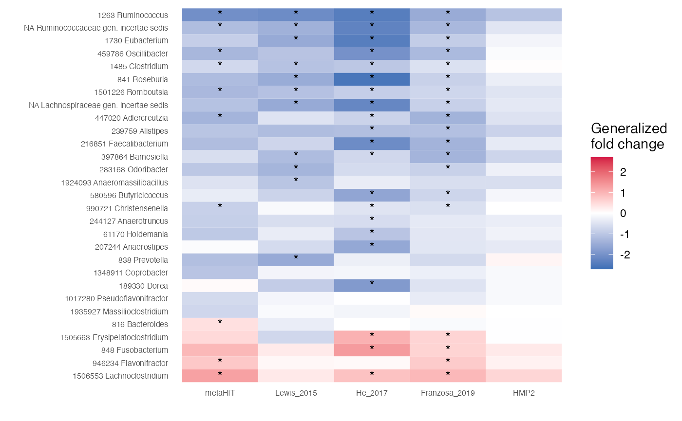
Now, we can compare the associations stored in the
df.assoc tibble. For example, we can extract features which
are very strongly associated with the label (single-feature AUROC >
0.75 or < 0.25) in at least one of the studies and plot the
generalized fold change as heatmap.
genera.of.interest <- df.assoc %>%
    group_by(genus) %>%
    summarise(m=mean(auc), n.filt=any(auc < 0.25 | auc > 0.75),
        .groups='keep') %>%
    filter(n.filt) %>%
    arrange(m)
After we extracted the genera, we plot them:
df.assoc %>%
    # take only genera of interest
    filter(genus %in% genera.of.interest$genus) %>%
    # convert to factor to enforce an ordering by mean AUC
    mutate(genus=factor(genus, levels = rev(genera.of.interest$genus))) %>%
    # convert to factor to enforce ordering again
    mutate(Study=factor(Study, levels = datasets)) %>%
    # annotate the cells in the heatmap with stars
    mutate(l=case_when(p.adj < 0.01~'*', TRUE~'')) %>%
    ggplot(aes(y=genus, x=Study, fill=fc)) +
        geom_tile() +
        scale_fill_gradient2(low = '#3B6FB6', high='#D41645', mid = 'white',
            limits=c(-2.7, 2.7), name='Generalized\nfold change') +
        theme_minimal() +
        geom_text(aes(label=l)) +
        theme(panel.grid = element_blank()) +
        xlab('') + ylab('') +
        theme(axis.text = element_text(size=6))
Study as Confounding Factor
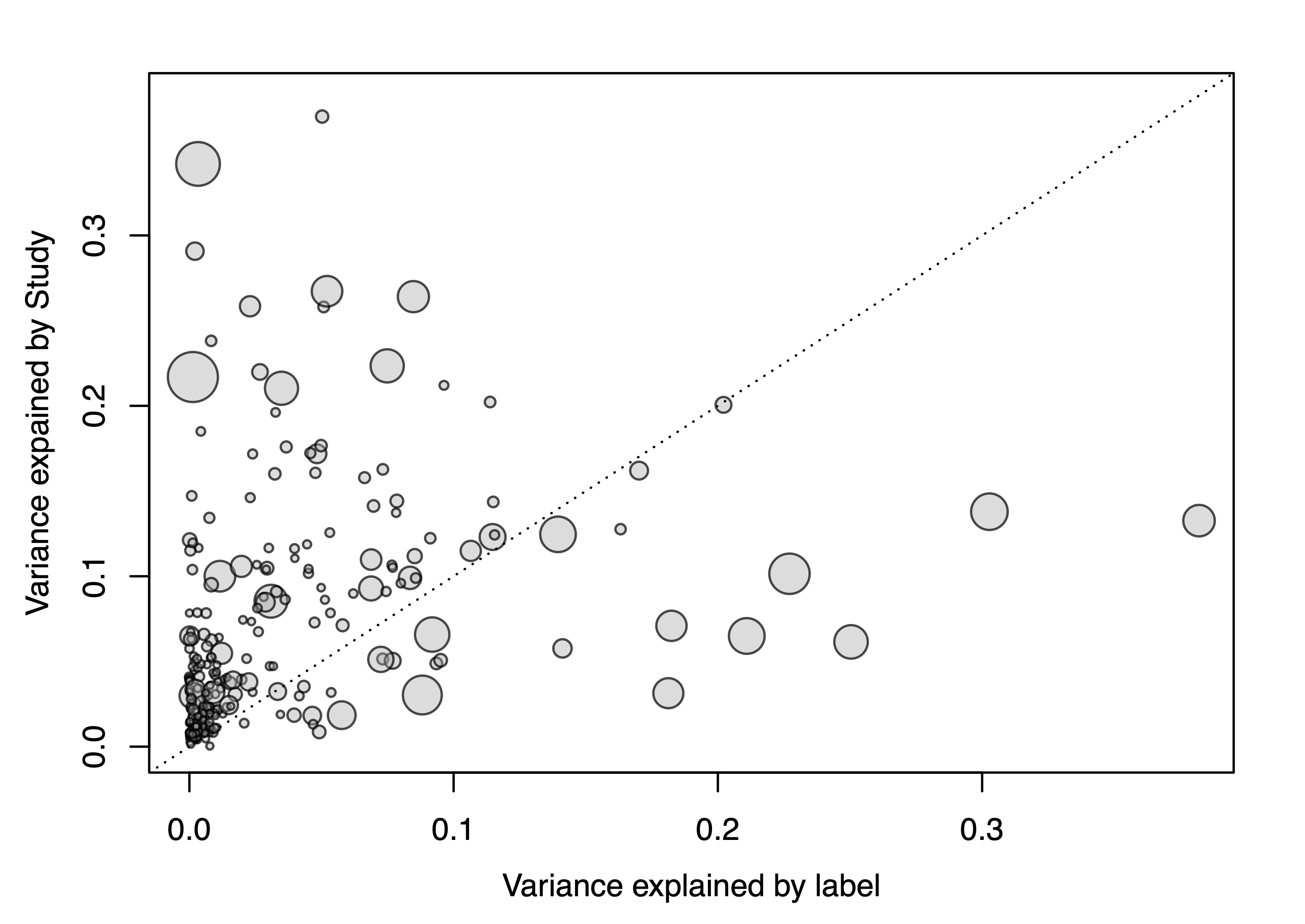
Additionally, we can check how differences between studies might
influence the variance of specific genera. To do so, we create a singel
SIAMCAT object which holds the complete datasets and then
we run the check.confounder function.
df.meta <- meta.ind %>%
    as.data.frame()
rownames(df.meta) <- df.meta$Sample_ID
sc.obj <- siamcat(feat=feat, meta=df.meta, label='Group', case='CD')
## + starting create.label
## Label used as case:
##    CD
## Label used as control:
##    CTR
## + finished create.label.from.metadata in    0 s
## + starting validate.data
## +++ checking overlap between labels and features
## + Keeping labels of 504 sample(s).
## +++ checking sample number per class
## +++ checking overlap between samples and metadata
## + finished validate.data in 0.262 s
check.confounders(sc.obj, fn.plot = './confounder_plot_cd_meta.pdf',
                feature.type='original')
## Finished checking metadata for confounders, results plotted to: ./confounder_plot_cd_meta.pdf
The resulting variance plot shows that some genera are strongly impacated by differences between studies, other genera not so much. Of note, the genera that vary most with the label (CD vs controls) do not show a lot of variance across studies.
ML Meta-analysis
Train LASSO Models
Lastly, we can perform the machine learning (ML) meta-analysis: we
first train one model for each datasets and then apply it to the other
datasets using the holdout testing functionality of
SIAMCAT. For datasets with repeated samples across
subjects, we block the cross-validation for subjects in order not to
bias the results (see also the vignette about Machine learning
pitfalls).
# create tibble to store all the predictions
auroc.all <- tibble(study.train=character(0),
                    study.test=character(0),
                    AUC=double(0))
# and a list to save the trained SIAMCAT objects
sc.list <- list()
for (i in datasets){
    # restrict to a single study
    meta.train <- meta.all %>%
        filter(Study==i) %>%
        as.data.frame()
    rownames(meta.train) <- meta.train$Sample_ID

    ## take into account repeated sampling by including a parameters
    ## in the create.data.split function
    ## For studies with repeated samples, we want to block the
    ## cross validation by the column 'Individual_ID'
    block <- NULL
    if (i %in% c('metaHIT', 'Lewis_2015', 'HMP2')){
        block <- 'Individual_ID'
        if (i == 'HMP2'){
            # for the HMP2 dataset, the number of repeated sample per subject
            # need to be reduced, because some subjects have been sampled
            # 20 times, other only 5 times
            meta.train <- meta.all %>%
                filter(Study=='HMP2') %>%
                group_by(Individual_ID) %>%
                sample_n(5, replace = TRUE) %>%
                distinct() %>%
                as.data.frame()
            rownames(meta.train) <- meta.train$Sample_ID
        }
    }
    # create SIAMCAT object
    sc.obj.train <- siamcat(feat=feat, meta=meta.train,
                            label='Group', case='CD')
    # normalize features
    sc.obj.train <- normalize.features(sc.obj.train, norm.method = 'log.std',
        norm.param=list(log.n0=1e-05, sd.min.q=0),feature.type = 'original')
    # Create data split
    sc.obj.train <- create.data.split(sc.obj.train,
        num.folds = 10, num.resample = 10, inseparable = block)
    # train LASSO model
    sc.obj.train <- train.model(sc.obj.train, method='lasso')

    ## apply trained models to other datasets

    # loop through datasets again
    for (i2 in datasets){
        if (i == i2){
            # make and evaluate cross-validation predictions (same dataset)
            sc.obj.train <- make.predictions(sc.obj.train)
            sc.obj.train <- evaluate.predictions(sc.obj.train)
            auroc.all <- auroc.all %>%
                add_row(study.train=i, study.test=i,
                    AUC=eval_data(sc.obj.train)$auroc %>% as.double())
        } else {
            # make and evaluate on the external datasets
            # use meta.ind here, since we want only one sample per subject!
            meta.test <- meta.ind %>%
                filter(Study==i2) %>%
                as.data.frame()
            rownames(meta.test) <- meta.test$Sample_ID
            sc.obj.test <- siamcat(feat=feat, meta=meta.test,
                                    label='Group', case='CD')
            # make holdout predictions
            sc.obj.test <- make.predictions(sc.obj.train,
                                            siamcat.holdout = sc.obj.test)
            sc.obj.test <- evaluate.predictions(sc.obj.test)
            auroc.all <- auroc.all %>%
                add_row(study.train=i, study.test=i2,
                    AUC=eval_data(sc.obj.test)$auroc %>% as.double())
        }
    }
    # save the trained model
    sc.list[[i]] <- sc.obj.train
}
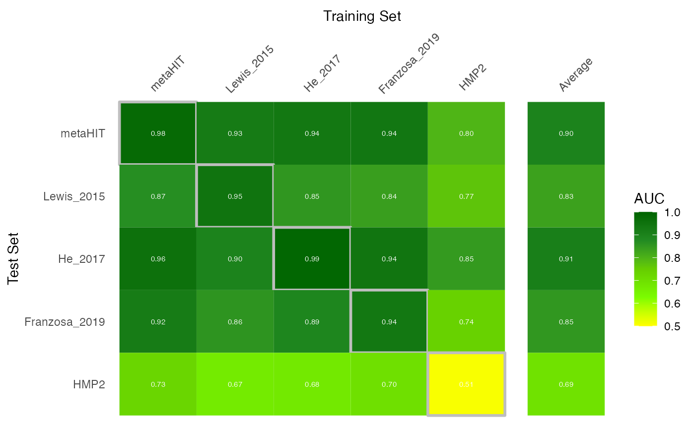
After we trained and applied all models, we can calculate the test average for each dataset:
test.average <- auroc.all %>%
    filter(study.train!=study.test) %>%
    group_by(study.test) %>%
    summarise(AUC=mean(AUC), .groups='drop') %>%
    mutate(study.train="Average")
Now that we have the AUROC values, we can plot them into a nice heatmap:
# combine AUROC values with test average
bind_rows(auroc.all, test.average) %>%
    # highlight cross validation versus transfer results
    mutate(CV=study.train == study.test) %>%
    # for facetting later
    mutate(split=case_when(study.train=='Average'~'Average', TRUE~'none')) %>%
    mutate(split=factor(split, levels = c('none', 'Average'))) %>%
    # convert to factor to enforce ordering
    mutate(study.train=factor(study.train, levels=c(datasets, 'Average'))) %>%
    mutate(study.test=factor(study.test,
                            levels=c(rev(datasets),'Average'))) %>%
    ggplot(aes(y=study.test, x=study.train, fill=AUC, size=CV, color=CV)) +
        geom_tile() + theme_minimal() +
        # text in tiles
        geom_text(aes_string(label="format(AUC, digits=2)"),
            col='white', size=2)+
        # color scheme
        scale_fill_gradientn(colours=rev(c('darkgreen','forestgreen',
                                        'chartreuse3','lawngreen',
                                        'yellow')), limits=c(0.5, 1)) +
        # axis position/remove boxes/ticks/facet background/etc.
        scale_x_discrete(position='top') +
        theme(axis.line=element_blank(),
                axis.ticks = element_blank(),
                axis.text.x.top = element_text(angle=45, hjust=.1),
                panel.grid=element_blank(),
                panel.border=element_blank(),
                strip.background = element_blank(),
                strip.text = element_blank()) +
        xlab('Training Set') + ylab('Test Set') +
        scale_color_manual(values=c('#FFFFFF00', 'grey'), guide=FALSE) +
        scale_size_manual(values=c(0, 1), guide=FALSE) +
        facet_grid(~split, scales = 'free', space = 'free')
## Warning: `aes_string()` was deprecated in ggplot2 3.0.0.
## ℹ Please use tidy evaluation ideoms with `aes()`
## This warning is displayed once every 8 hours.
## Call `lifecycle::last_lifecycle_warnings()` to see where this warning was
## generated.
## Warning: Using `size` aesthetic for lines was deprecated in ggplot2 3.4.0.
## ℹ Please use `linewidth` instead.
## This warning is displayed once every 8 hours.
## Call `lifecycle::last_lifecycle_warnings()` to see where this warning was
## generated.
## Warning: The `guide` argument in `scale_*()` cannot be `FALSE`. This was deprecated in
## ggplot2 3.3.4.
## ℹ Please use "none" instead.
## This warning is displayed once every 8 hours.
## Call `lifecycle::last_lifecycle_warnings()` to see where this warning was
## generated.
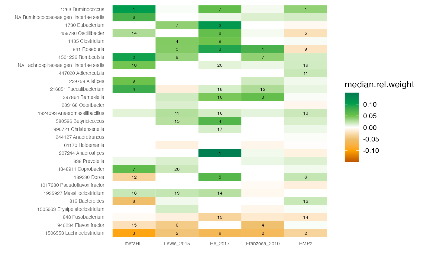
Investigate Feature Weights
Now that we the trained models (and we saved them in the
sc.list object), we can also extract the model weights
using SIAMCAT and compare to the associations we computed
above.
weight.list <- list()
for (d in datasets){
    sc.obj.train <- sc.list[[d]]
    # extract the feature weights out of the SIAMCAT object
    temp <- feature_weights(sc.obj.train)
    temp$genus <- rownames(temp)
    # save selected info in the weight.list
    weight.list[[d]] <- temp %>%
        select(genus, median.rel.weight, mean.rel.weight, percentage) %>%
        mutate(Study=d) %>%
        mutate(r.med=rank(-abs(median.rel.weight)),
            r.mean=rank(-abs(mean.rel.weight)))
}
# combine all feature weights into a single tibble
df.weights <- bind_rows(weight.list)
df.weights <- df.weights %>% filter(genus!='unclassified')
Using this, we can plot another heatmap with the weights, focussing on the genera of interest for which we plotted the associations as heatmap above.
# compute absolute feature weights
abs.weights <- df.weights %>%
    group_by(Study) %>%
    summarise(sum.median=sum(abs(median.rel.weight)),
                sum.mean=sum(abs(mean.rel.weight)),
                .groups='drop')

df.weights %>%
    full_join(abs.weights) %>%
    # normalize by the absolute model size
    mutate(median.rel.weight=median.rel.weight/sum.median) %>%
    # only include genera of interest
    filter(genus %in% genera.of.interest$genus) %>%
    # highlight feature rank for the top 20 features
    mutate(r.med=case_when(r.med > 20~NA_real_, TRUE~r.med)) %>%
    # enforce the correct ordering by converting to factors again
    mutate(genus=factor(genus, levels = rev(genera.of.interest$genus))) %>%
    mutate(Study=factor(Study, levels = datasets)) %>%
    ggplot(aes(y=genus, x=Study, fill=median.rel.weight)) +
        geom_tile() +
        scale_fill_gradientn(colours=rev(
            c('#007A53', '#009F4D', "#6CC24A", 'white',
            "#EFC06E", "#FFA300", '#BE5400')),
            limits=c(-0.15, 0.15)) +
        theme_minimal() +
        geom_text(aes(label=r.med), col='black', size= 2) +
        theme(panel.grid = element_blank()) +
        xlab('') + ylab('') +
        theme(axis.text = element_text(size=6))
## Joining with `by = join_by(Study)`
Session Info
sessionInfo()
## R version 4.2.2 (2022-10-31)
## Platform: x86_64-apple-darwin17.0 (64-bit)
## Running under: macOS Big Sur ... 10.16
##
## Matrix products: default
## BLAS:   /Library/Frameworks/R.framework/Versions/4.2/Resources/lib/libRblas.0.dylib
## LAPACK: /Library/Frameworks/R.framework/Versions/4.2/Resources/lib/libRlapack.dylib
##
## locale:
## [1] en_US.UTF-8/en_US.UTF-8/en_US.UTF-8/C/en_US.UTF-8/en_US.UTF-8
##
## attached base packages:
## [1] stats     graphics  grDevices utils     datasets  methods   base
##
## other attached packages:
##  [1] SIAMCAT_2.3.3    phyloseq_1.42.0  mlr3_0.14.1      lubridate_1.9.2
##  [5] forcats_1.0.0    stringr_1.5.0    dplyr_1.1.0      purrr_1.0.1
##  [9] readr_2.1.4      tidyr_1.3.0      tibble_3.2.0     ggplot2_3.4.1
## [13] tidyverse_2.0.0  BiocStyle_2.26.0
##
## loaded via a namespace (and not attached):
##   [1] uuid_1.1-0             backports_1.4.1        corrplot_0.92
##   [4] systemfonts_1.0.4      plyr_1.8.8             igraph_1.4.1
##   [7] splines_4.2.2          listenv_0.9.0          GenomeInfoDb_1.34.9
##  [10] gridBase_0.4-7         digest_0.6.31          foreach_1.5.2
##  [13] htmltools_0.5.4        lmerTest_3.1-3         fansi_1.0.4
##  [16] magrittr_2.0.3         checkmate_2.1.0        memoise_2.0.1
##  [19] cluster_2.1.4          tzdb_0.3.0             globals_0.16.2
##  [22] Biostrings_2.66.0      mlr3tuning_0.18.0      matrixStats_0.63.0
##  [25] vroom_1.6.1            timechange_0.2.0       pkgdown_2.0.7
##  [28] prettyunits_1.1.1      colorspace_2.1-0       textshaping_0.3.6
##  [31] xfun_0.37              crayon_1.5.2           RCurl_1.98-1.10
##  [34] jsonlite_1.8.4         lme4_1.1-32            survival_3.5-5
##  [37] iterators_1.0.14       ape_5.7-1              glue_1.6.2
##  [40] gtable_0.3.1           zlibbioc_1.44.0        XVector_0.38.0
##  [43] Rhdf5lib_1.20.0        shape_1.4.6            BiocGenerics_0.44.0
##  [46] scales_1.2.1           infotheo_1.2.0.1       DBI_1.1.3
##  [49] Rcpp_1.0.10            progress_1.2.2         palmerpenguins_0.1.1
##  [52] bit_4.0.5              stats4_4.2.2           glmnet_4.1-6
##  [55] RColorBrewer_1.1-3     ellipsis_0.3.2         farver_2.1.1
##  [58] pkgconfig_2.0.3        sass_0.4.5             utf8_1.2.3
##  [61] labeling_0.4.2         tidyselect_1.2.0       rlang_1.1.0
##  [64] reshape2_1.4.4         PRROC_1.3.1            munsell_0.5.0
##  [67] tools_4.2.2            cachem_1.0.7           cli_3.6.0
##  [70] generics_0.1.3         ade4_1.7-22            evaluate_0.20
##  [73] biomformat_1.26.0      fastmap_1.1.1          yaml_2.3.7
##  [76] ragg_1.2.5             bit64_4.0.5            knitr_1.42
##  [79] fs_1.6.1               lgr_0.4.4              beanplot_1.3.1
##  [82] bbotk_0.7.2            future_1.32.0          nlme_3.1-162
##  [85] paradox_0.11.0         compiler_4.2.2         rstudioapi_0.14
##  [88] curl_5.0.0             bslib_0.4.2            stringi_1.7.12
##  [91] highr_0.10             desc_1.4.2             lattice_0.20-45
##  [94] Matrix_1.5-3           nloptr_2.0.3           vegan_2.6-4
##  [97] permute_0.9-7          multtest_2.54.0        vctrs_0.5.2
## [100] pillar_1.8.1           lifecycle_1.0.3        rhdf5filters_1.10.0
## [103] BiocManager_1.30.20    jquerylib_0.1.4        LiblineaR_2.10-22
## [106] data.table_1.14.8      bitops_1.0-7           R6_2.5.1
## [109] bookdown_0.33          gridExtra_2.3          mlr3misc_0.11.0
## [112] IRanges_2.32.0         parallelly_1.34.0      codetools_0.2-19
## [115] boot_1.3-28.1          MASS_7.3-58.3          rhdf5_2.42.0
## [118] mlr3learners_0.5.6     rprojroot_2.0.3        withr_2.5.0
## [121] S4Vectors_0.36.2       GenomeInfoDbData_1.2.9 mgcv_1.8-42
## [124] parallel_4.2.2         hms_1.1.2              grid_4.2.2
## [127] minqa_1.2.5            rmarkdown_2.20         pROC_1.18.0
## [130] numDeriv_2016.8-1.1    Biobase_2.58.0